NVIDIA Jetson Edge AI Whitepaper 30. August 2026 8 Min. Lesezeit

KI auf NVIDIA Jetson mit einer kleineren Runtime statt einem kleineren Modell

Gemessene Ergebnisse aus dem Neubau des Inferenz- und Video-Stacks für NVIDIA Jetson.

Autor: Gary Hilgemann, REBOTNIX
Messplattform: NVIDIA Jetson Orin NX 16 GB auf REBOTNIX Blade, JetPack 6.2 (L4T R36.5)
Version 1, Ergebniszusammenfassung. Der technische Report mit den Methoden hinter diesen Zahlen ist auf Anfrage erhältlich, siehe Ende dieses Artikels.

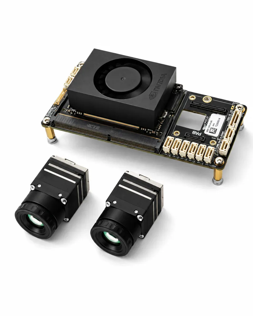
REBOTNIX Blade mit NVIDIA Jetson Orin NX Modul und zwei angeschlossenen Kameras

Das Testsystem: NVIDIA Jetson Orin NX 16 GB auf REBOTNIX Blade.

Gemessen auf NVIDIA Jetson Orin NX

501 MB

vollständige Detektions-Pipeline, Spitzenwert resident

6,92 ms

Inferenz pro Bild: 145 fps Inferenz-Durchsatz, 104 fps Ende zu Ende inkl. H.264-Decode

1,4 GB

freigemacht bei vier Modellen, ohne Modelländerung

82 mJ

zusätzliche Boardenergie pro inferiertem Bild, Ende zu Ende

Das Problem an der üblichen Dimensionierung von Edge AI

Wer ein funktionierendes Modell auf ein Embedded-Modul gebracht hat, kennt den Moment. Auf der Workstation ist es genau und schnell. Auf dem Zielsystem passt es nicht, die Bildrate bleibt hinter dem zurück, was die Anwendung braucht, und das zweite Modell war ohnehin nie realistisch.

Das ist keine Grenze der Hardware. NVIDIA Jetson Module haben die Rechenleistung. Das Problem ist, dass der größte Teil des Software-Stacks darüber nie für ein festes Speicherbudget geschrieben wurde. Desktop-Frameworks setzen Page Cache, Swap und eine diskrete GPU mit eigenem Speicher voraus. Auf einem Jetson teilen sich CPU und GPU einen physischen Speicherpool, und jedes Byte, das ein Framework aus Bequemlichkeit hält, ist ein Byte, das dem neuronalen Netz fehlt.

Die übliche Antwort ist, das Modell zu verkleinern: eine kleinere Variante, INT8, Pruning, geringere Auflösung. Das funktioniert, und es geht schnell. Es verändert aber auch, was das Netz ausgibt. Damit muss das Wahrnehmungsmodell des Kunden neu getestet und in einer regulierten Domäne neu zertifiziert werden.

Wir sind den anderen Weg gegangen: Wir haben die Runtime neu gebaut, statt das Modell zu verkleinern.

Warum der Speicher selten im Modell steckt

Bevor man etwas optimiert, lohnt es sich zu wissen, was auf einem Jetson zur Inferenzzeit tatsächlich Speicher hält. Wir haben unseren eigenen Detektionsprozess vom Kaltstart bis in den eingeschwungenen Zustand instrumentiert und den residenten Speicher in jeder Stufe gemessen. Die Last ist ein einstufiger Detektor, 640x640 Eingabe, FP16 TensorRT Engine, 80 Klassen.

Abbildung 1 · Wohin der Speicher geht (gemessen)

Zuwachs je Stufe, vom Kaltstart bis in den eingeschwungenen Zustand. Die Engine selbst ist der kleinste Posten im Bild.

Lesen Sie die Zuwächse, denn sie stellen die ganze Diskussion neu auf.

Die FP16 Engine auf der Festplatte ist 21 MB groß. Sie auf INT8 zu quantisieren spart davon rund 10 MB, also unter zwei Prozent eines 538 MB großen Prozesses, im Tausch gegen eine Kalibrierungskampagne und ein Gespräch mit dem Kunden über Genauigkeit.

Die beiden großen Sprünge sind der CUDA-Kontext mit der hochfahrenden TensorRT Runtime (283 MB) und die Allokation beim Warmup (177 MB), in der Aktivierungsspeicher, Device-I/O-Puffer und die beim ersten Aufruf nachgeladenen CUDA-Module stecken. Die erste Zahl rührt Quantisierung überhaupt nicht an. Von der zweiten kann sie den Aktivierungsanteil verkleinern, nicht aber die Runtime-Module und nicht den Kontext, und in diesem Profil sind genau diese festen Kosten der größere Block. Sie werden kleiner, wenn Sie aufhören, ein zweites Framework darüber zu instanziieren, wenn Sie aufhören, pro Prozess einen eigenen CUDA-Kontext zu bezahlen, und wenn Sie aufhören, Puffer zu allokieren, die Sie nicht verwenden.

Genau dorthin ist unsere Entwicklungsarbeit gegangen.

Was wir gemessen haben

KINEVA ist eine native C++ Inferenz-Engine, rb_vision eine native C Video-Pipeline, beide von Grund auf für Jetson geschrieben. Alle folgenden Zahlen wurden auf dem oben genannten Modul erhoben, im vollen Power-Modus, mit tegrastats über die exakte Dauer jedes Laufs.

Eine vollständige Detektions-Pipeline in 501 MB

501 MB Spitzenwert an residentem Speicher für den gesamten Pfad, also CUDA-Kontext, TensorRT Runtime, Engine-Gewichte, Video-Dekodierung, Vorverarbeitung, Inferenz und NMS, bei 6,92 ms Inferenz pro Bild: 145 fps Inferenz-Durchsatz, 104 fps Ende zu Ende einschließlich H.264-Decode auf 720p Video. Der Kaltstart kostet 1,17 s Engine-Ladezeit plus 67 ms Warmup, einmalig.

Der Detektor-Output ist unverändert. Keine Quantisierung unter FP16, kein Pruning, keine Reduktion der Auflösung. Gegen die PyTorch-Referenz validiert, auf subpixelgenaue Boxen und drei Nachkommastellen der Konfidenz.

Abbildung 2 · Was tatsächlich ausgeliefert wird (gemessen, auf der Festplatte)

Logarithmische Achse, sonst verschwindet die 1,5 MB große Binary neben dem versiegelten Modellpaket.

Kein Interpreter, kein ML-Framework, kein Media-Framework auf dem Zielsystem. Es gibt keine Python-Umgebung, die gepinnt werden muss, keine Framework-Version, die über JetPack-Upgrades hinweg nachgehalten werden muss, und keinen Dependency-Drift im Feld.

Vier Modelle auf einem Modul zum Preis von anderthalb

Die meisten realen Anwendungen betreiben mehr als ein Modell, und das übliche Muster ist ein Prozess pro Modell. Auf Jetson ist dieses Muster teuer, aus einem Grund, der nichts mit den Modellen zu tun hat: jeder Prozess bezahlt seinen eigenen CUDA-Kontext und seine eigene TensorRT Runtime, rund 350 MB, bevor ein einziges Gewicht geladen ist.

Wir haben vier im Haus trainierte Detektoren in einen einzigen Prozess gelegt, alle warm und pro Bild adressierbar:

kineva_coco, allgemeine Detektion über 80 Klassen
illegalwaste, Erkennung illegaler Müllablagerung
head, Kopf- und Personenerkennung
licenseplate, Kennzeichenerkennung

Abbildung 3 · Vier Modelle, ein Prozess gegenüber vier Prozessen (gemessen)

Die gemeinsame Basis wird einmal bezahlt. Jeder weitere resident gehaltene Detektor kostet dann 43 bis 107 MB statt eines weiteren vollständigen Stacks.

1,4 GB auf einem Modul freigemacht, ohne Änderung an einem einzigen Modell. Auf einem 4-GB-Modul ist dieser Unterschied das gesamte Deployment.

82 Millijoule pro inferiertem Bild

Erfasst mit tegrastats in 500-ms-Intervallen über einen durchgehenden Lauf von 1200 Bildern, 104 fps Ende zu Ende einschließlich H.264-Decode.

Abbildung 4 · Dauerbetrieb: Speicher, GPU-Auslastung und Boardleistung (gemessen)

System RAM (MB)

GPU-Auslastung (%)

VDD_IN Boardleistung (mW)

VDD_CPU_GPU_CV (mW)

Leerlauf gegenüber Dauerlast. Vier Größen auf vier verschiedenen Skalen, deshalb vier getrennte Paare statt einer gemeinsamen Achse.

8,5 W zusätzliche Boardleistung bei 104 fps Ende zu Ende sind 82 mJ pro inferiertem Bild, eine Größe, die ein Flottenplaner hochrechnen kann. Geteilt durch die reine Inferenzrate ergäbe sich eine geschmeichelte 58, wir nennen die Ende-zu-Ende-Zahl, weil das Deployment die Ende-zu-Ende-Zahl bezahlt. Und bei 62 % durchschnittlicher GPU-Auslastung ist das Modul nicht ausgelastet: Es bleibt Luft für eine zweite Last auf demselben Silizium, und genau das macht ein kleineres Modul zu einem realistischen Ziel statt zu einer Hoffnung.

Eine Feldnotiz, kostenlos für das Ökosystem

Dieser Punkt hat uns echte Zeit gekostet. Er ist eine Eigenschaft der Plattform und keine Methode von uns, deshalb veröffentlichen wir ihn.

Setzen Sie den Power-Modus, bevor Sie irgendetwas messen. Unsere erste Dual-Stream-Messung entstand versehentlich im 15-W-Modus: vier von acht Kernen online, gedeckelt bei 1,42 GHz. Sie las 33,5 fps pro Stream, und wir schlossen daraus, dass das Ziel nicht erreichbar sei. Im vollen Power-Modus hält derselbe Code 110,7 fps. Eine einzige nvpmodel-Einstellung hat ein Engineering-Urteil umgedreht und uns beinahe eine Produktentscheidung gekostet.

Zur Ehrlichkeit im Berichten

Zwei Gewohnheiten, weil sie der Grund dafür sind, dass man den obigen Zahlen trauen kann.

Wir veröffentlichen Ergebnisse, die gegen unsere eigene Erwartung ausfielen. Dieselbe Engine und dieselben 300 Bilder einmal über die native CLI und einmal über die Python-Bindings gemessen ergaben 501 MB gegenüber 541 MB, also 40 MB Unterschied (rund 8 %) und 1,4 % Latenz. Die Aussage "wir haben Python entfernt und Gigabytes gespart" ist damit durch die Messung nicht gedeckt, und wir treffen sie nicht. Der Interpreter ist billig, das Framework ist teuer. Entfernt haben wir das ML-Framework aus dem Inferenzpfad, nicht die Sprache. Die Bindings existieren, damit Integrationscode in Python bleiben kann, während der speicherrelevante Teil nativ ist.

Wir haben außerdem zwei eigene Optimierungen dokumentiert, die schlechter maßen als die Ausgangsversion, und sie auf Basis der Evidenz verworfen, statt sie auf Basis einer Annahme weiterzuverfolgen. Beide stehen im technischen Report, mitsamt der Instrumentierung dahinter.

Warum das von REBOTNIX kommt

Drei Eigenschaften ergeben sich daraus, den gesamten Stack zu besitzen statt einer Schicht davon.

Wir liefern das vollständige System, nicht eine Komponente. Kamera-Hardware, Carrier-Integration, die Inferenz-Engine, die Modelle, die Video-Pipeline, Lizenzierung und IP-Schutz, aus einer Hand und über einen Supportweg. Speicher- und Leistungsverhalten sind damit Entwicklungsentscheidungen, die wir auf das Budget eines Kunden zubewegen können, und keine Eigenschaften eines Frameworks, um die wir herumarbeiten müssen.

Die Modelle gehören uns. Die vier gemessenen Detektoren sind kein Sonderfall, sondern ein Ausschnitt aus der Palette, die vollständig im Haus trainiert wird:

KINEVA CNN

Kopf- und Personenerkennung
Kennzeichenerkennung
Erkennung illegaler Entsorgung
Abfallkategorie
PKW- und LKW-Erkennung
COCO 80-Klassen
Graffiti-Erkennung
Verkehrszeichenerkennung
Gesichtsanonymisierung

KINEVA PCNN

WiFi Person Scanner
Virtual RTK GPS
Fahrzeugerkennung und Klassifizierung
Flugzeugerkennung
Schiffs- und Maritimerkennung
Multi-Sensor Flugverfolgung

KINEVA VLLM und LLM

Industrial Scene Understanding
Infrastructure Report Generator

Siebzehn Modelle, drei Familien, eine Runtime. Details unter KINEVA.

In der Runtime steckt kein fremder Inferenz-Wrapper. Der Kunde erbt damit keine Copyleft-Verpflichtung aus dem Wahrnehmungs-Stack. Auf der Video-Seite haben wir dieselbe Überlegung angewandt und einen permissiv lizenzierten Software-Encoder gegenüber der GPL-Alternative gewählt, damit das Produkt closed-source ausgeliefert werden kann.

IP-Schutz ist Teil der Runtime. Modelle werden AES/ChaCha versiegelt ausgeliefert und im Speicher gegen ihren registrierten Namen entschlüsselt. Lizenzierung und Maschinenbindung sind in die Engine eingebaut, ohne OpenSSL auf dem Zielsystem.

Version 2 · Unter NDA

Den technischen Report anfordern

Dieser Artikel berichtet, was wir erreicht haben. Ein zweites Dokument beschreibt, wie, und ist auf Anfrage unter NDA erhältlich:

Die acht Runtime-Techniken hinter den obigen Zahlen, jeweils mit gemessener Wirkung und Trade-off
Das Host-Staging pro Bild, das aus dem Inferenzpfad entfernt wurde, und wie
Die Verteilung der Arbeit über das SoC, also welche Pipeline-Stufe auf welcher Engine läuft und was jede Verschiebung gekostet oder gespart hat
Die zwei Optimierungen, die schlechter maßen als die Ausgangsversion, mit der Instrumentierung, die es gezeigt hat
Die Residenz-Architektur hinter den 1,4 GB und die Entscheidungskurve zwischen Nachladen und Residenz
Vollständige Reproduktionsbefehle für jede Messung in beiden Dokumenten

Sie arbeiten an einem Jetson-Deployment, das nicht in das geplante Modul passt? Die Antwort ist nicht immer ein kleineres Modell. Sehr oft ist es eine kleinere Runtime. Bringen Sie uns die Last und das Modul, auf dem sie laufen soll.

Alle Messwerte beziehen sich auf die oben genannte Konfiguration und können je nach Hardware, Software-Stand und Last abweichen. Änderungen und Irrtümer vorbehalten.

Alle Beiträge Kontakt aufnehmen

Back to Blog

NVIDIA Jetson Edge AI Whitepaper 30 August 2026 8 min read

Running AI on NVIDIA Jetson with a Smaller Runtime, Not a Smaller Model

Measured results from rebuilding the inference and video stack for NVIDIA Jetson.

Author: Gary Hilgemann, REBOTNIX
Platform of record: NVIDIA Jetson Orin NX 16 GB on REBOTNIX Blade, JetPack 6.2 (L4T R36.5)
Version 1, results summary. The technical report covering the methods behind these numbers is available on request, see the end of this document.

REBOTNIX Blade carrying an NVIDIA Jetson Orin NX module with two attached cameras

The test system: NVIDIA Jetson Orin NX 16 GB on REBOTNIX Blade.

Measured on NVIDIA Jetson Orin NX

501 MB

complete detection pipeline, peak resident

6.92 ms

inference per frame: 145 fps inference throughput, 104 fps end to end incl. H.264 decode

1.4 GB

freed across four models, no model changed

82 mJ

incremental board energy per inferred frame, end to end

The Problem With How Edge AI Usually Gets Sized

If you have moved a working model onto an embedded module, you know the moment. On the workstation it is accurate and fast. On the target it does not fit, the frame rate is short of what the application needs, and the second model was never going to happen.

This is not a limitation of the hardware. NVIDIA Jetson modules have the compute. The problem is that most of the software stack on top of them was never written for a fixed memory budget. Desktop frameworks assume page cache, swap, and a discrete GPU with memory of its own. On a Jetson the CPU and GPU share one physical pool, and every byte a framework holds for convenience is a byte the neural network cannot use.

The usual response is to shrink the model: a smaller variant, INT8, pruning, lower resolution. It works, and it is quick. It also changes what the network outputs, which means the customer's perception model has to be re-tested and, in a regulated domain, re-certified.

We took the other route: we rebuilt the runtime instead of shrinking the model.

Why the Model Is Rarely Where the Memory Is

Before optimizing anything, it is worth knowing what actually holds memory on a Jetson at inference time. We instrumented our own detection process from a cold start through to steady-state inference and measured resident memory at each stage. The workload is a single-stage detector, 640x640 input, FP16 TensorRT engine, 80 classes.

Figure 1 · Where the memory goes in a complete detection pipeline (measured)

Increment per stage, from cold start to steady state. The engine itself is the smallest item on the chart.

Read the increments, because they reframe the whole discussion.

The FP16 engine on disk is 21 MB. Quantizing it to INT8 would save roughly 10 MB of that, under two percent of a 538 MB process, in exchange for a calibration campaign and an accuracy conversation with the customer.

The two large jumps are the CUDA context with the TensorRT runtime coming up (283 MB), and the warmup allocation (177 MB), which covers activation memory, device I/O buffers, and the CUDA modules loaded on first use. Quantization does not touch the first number at all. It can shrink the activation share of the second, but not the runtime modules and not the context, and on this profile those fixed costs are the bulk of the process. They get smaller when you stop instantiating a second framework on top of them, stop paying for a CUDA context per process, and stop allocating buffers you are not using.

That is where our engineering went.

What We Measured

KINEVA is a native C++ inference engine and rb_vision a native C video pipeline, both written from scratch for Jetson. All figures below were taken on the module named at the top of this document, in full power mode, with tegrastats sampled for the exact duration of each run.

A complete detection pipeline in 501 MB

501 MB peak resident memory for the full path, covering CUDA context, TensorRT runtime, engine weights, video decode, preprocessing, inference and NMS, at 6.92 ms inference per frame: 145 fps inference throughput, 104 fps end to end including H.264 decode on 720p video. Cold start is 1.17 s engine load plus 67 ms warmup, one time.

The detector output is unchanged. No quantization below FP16, no pruning, no resolution reduction. Validated against the PyTorch reference to sub-pixel boxes and three decimal places of confidence.

Figure 2 · What actually gets deployed (measured, on disk)

Logarithmic axis, otherwise the 1.5 MB binary disappears next to the sealed model package.

No interpreter, no ML framework, no media framework on the target. There is no Python environment to pin, no framework version to track across JetPack upgrades, and no dependency drift in the field.

Four models on one module for the price of one and a half

Most real applications run more than one model, and the common pattern is one process per model. On Jetson that pattern is expensive for a reason unrelated to the models: every process pays for its own CUDA context and TensorRT runtime, roughly 350 MB, before a single weight is loaded.

We put four detectors trained in-house into a single process, all warm and routable per frame:

kineva_coco, 80-class general detection
illegalwaste, illegal waste dumping
head, head and person detection
licenseplate, licence plate detection

Figure 3 · Four models, one process versus four processes (measured)

The shared base is paid once. Each additional resident detector then costs 43 to 107 MB rather than another full stack.

1.4 GB freed on one module, with no change to any model. On a 4 GB module, that difference is the entire deployment.

82 millijoules per inferred frame

Sampled with tegrastats at 500 ms intervals across a continuous 1200-frame run, 104 fps end to end including H.264 decode.

Figure 4 · Sustained detection: memory, GPU utilisation and board power (measured)

System RAM (MB)

GPU utilisation (%)

VDD_IN board power (mW)

VDD_CPU_GPU_CV (mW)

Idle versus sustained load. Four metrics on four different scales, so four separate pairs rather than one shared axis.

8.5 W of incremental board power at 104 fps end to end is 82 mJ per inferred frame, a figure a fleet planner can multiply out. Dividing by the inference-only rate would flatter that to 58; we report the end-to-end figure, because the end-to-end figure is what the deployment pays. And at 62 % average GPU utilisation the module is not saturated: there is headroom for a second workload on the same silicon, which is what makes a smaller module a realistic target rather than a hopeful one.

One Field Note, Free to the Ecosystem

This cost us real time to find. It is a platform property rather than a method of ours, so we are publishing it.

Set the power mode before you measure anything. Our first dual-stream measurement was taken accidentally in 15 W mode: four of eight cores online, capped at 1.42 GHz. It read 33.5 fps per stream and we concluded the target was unreachable. In full power mode the same code sustains 110.7. One nvpmodel setting inverted an engineering verdict and nearly cost us a product decision.

On Reporting Honestly

Two habits, because they are the reason the numbers above can be trusted.

We publish results that went against our own expectations. Measuring the same engine and the same 300 frames through the native CLI and through the Python bindings gave 501 MB versus 541 MB, a difference of 40 MB (about 8 %) and 1.4 % latency. So the claim "we removed Python and saved gigabytes" is not supported by measurement, and we do not make it. The interpreter is cheap; the framework is expensive. What we removed is the ML framework from the inference path, not the language. The bindings exist so integration code can stay in Python while the memory-relevant part is native.

We also documented two optimizations of our own that measured worse than the baseline and were abandoned on the evidence rather than pursued on the assumption. Both are in the technical report, with the instrumentation behind them.

Why This Comes From REBOTNIX

Three properties fall out of owning the whole stack rather than a layer of it.

We deliver the complete system, not a component. Camera hardware, carrier integration, the inference engine, the models, the video pipeline, licensing and IP protection, from one source, on one support path. Memory and power behaviour are therefore engineering decisions we can move to fit a customer's budget, not properties of a framework we have to work around.

The models are ours. The four detectors measured here are not a special case. They are a slice of a catalogue that is trained in-house end to end:

KINEVA CNN

Head / Person Detection
License Plate Detection
Illegal Waste Detection
Waste Category
Car / Truck Detection
COCO 80-Class
Graffiti Detection
Traffic Sign Recognition
Face Anonymisation

KINEVA PCNN

WiFi Person Scanner
Virtual RTK GPS
Vehicle Detection and Classification
Aircraft Detection
Ship and Maritime Detection
Multi-Sensor Flight Tracking

KINEVA VLLM and LLM

Industrial Scene Understanding
Infrastructure Report Generator

Seventeen models, three families, one runtime. Details at KINEVA.

There is no third-party inference wrapper anywhere in the runtime, so the customer inherits no copyleft obligation from the perception stack. We applied the same reasoning on the video side, selecting a permissively licensed software encoder over the GPL alternative specifically so the product can ship closed-source.

IP protection is part of the runtime. Models ship AES/ChaCha sealed and are decrypted in memory against their registered name; licensing and machine binding are built into the engine, with no OpenSSL on the target.

Version 2 · Under NDA

Request the technical report

This document reports what we achieved. A second document covers how, and is available on request under NDA:

The eight runtime techniques behind the figures above, each with its measured effect and its trade-off
The per-frame host staging that was eliminated from the inference path, and how
Work placement across the SoC, which pipeline stage runs on which engine, and what each move cost or saved
The two optimizations that measured worse than the baseline, with the instrumentation that showed it
The residency architecture behind the 1.4 GB, and the reload-versus-resident decision curve
Full reproduction commands for every measurement in both documents

Working on a Jetson deployment that does not fit the module you budgeted for? The answer is not always a smaller model. Very often it is a smaller runtime. Bring us the workload and the module you want it on.

All figures refer to the configuration named above and may differ with hardware, software revision and workload. Subject to change, errors and omissions excepted.

All posts Get in touch